This method for decision making is really old (Zangemeister
1973). Here, one common scale of values is used, that is not based on
monetary values. Instead, one uses scores like in school.
Every criterion must be rated according to those scores.
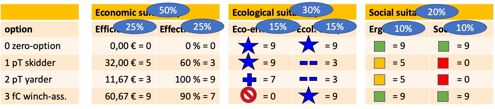
Next, one gives a weight to every
criterion according to its relative importance. The sum of weights should be
1.0
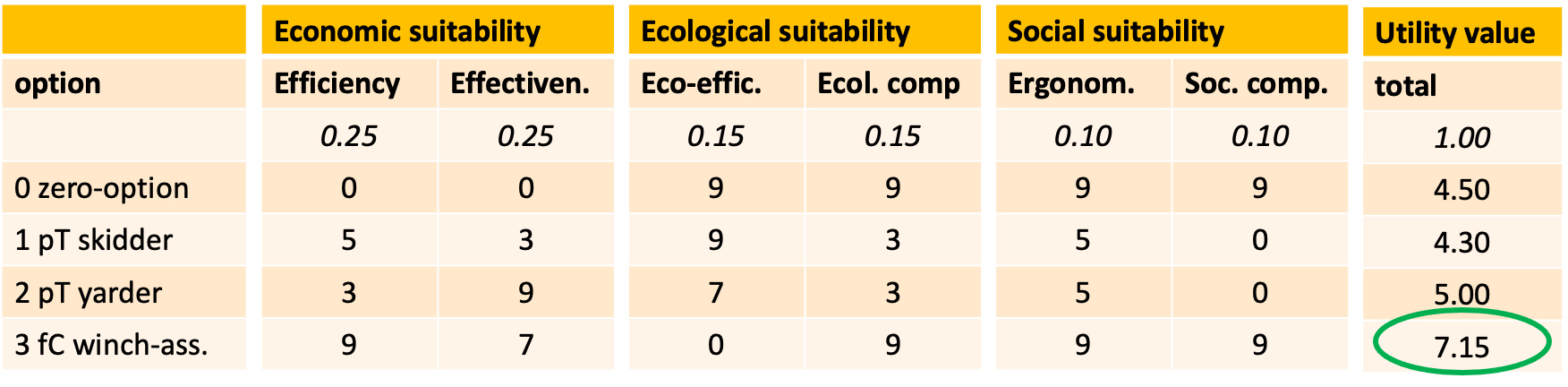
Finally, each score is multiplied by the
respective weight and then summed up. The option with the highest score will be
the favorite.
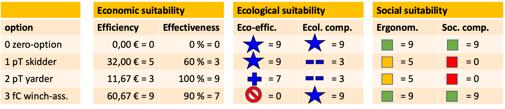
Let’s take an example. Here we introduce a value scale with scores that allow a rough assessment like:
9 = very good
7 = good, better than average
5 = expected average
3 = borderline, but not the worst
0 = not acceptable
Then we need some weights for the
different criteria. It is easier to weigh the three main pillars first, for example
The result is quickly told: again, option
3 CTL (hC
winch-assist) wins, option 1 is a bit worst than the zero-option. No option is really bad, but also no
option is extraordinarily good (the range of values is between 4.3 and 7.15). This is one of the disadvantages of this
method: It equalizes all options near the center.
Scientists do not rate this analytical
method too high, because it has a couple of mathematical bugs, that make it
unscholarly. One of the most relevant critics at the
utility analysis is, that it uses mathematical operations that are not
rational. In particular, the scores 0-9 are data on
an ordinary scale, which only knows “more”, “equal” and “less”. Operations like
adding or multiplying may not be done.
But it has one advantage: It allows for a transparent decision-making process.