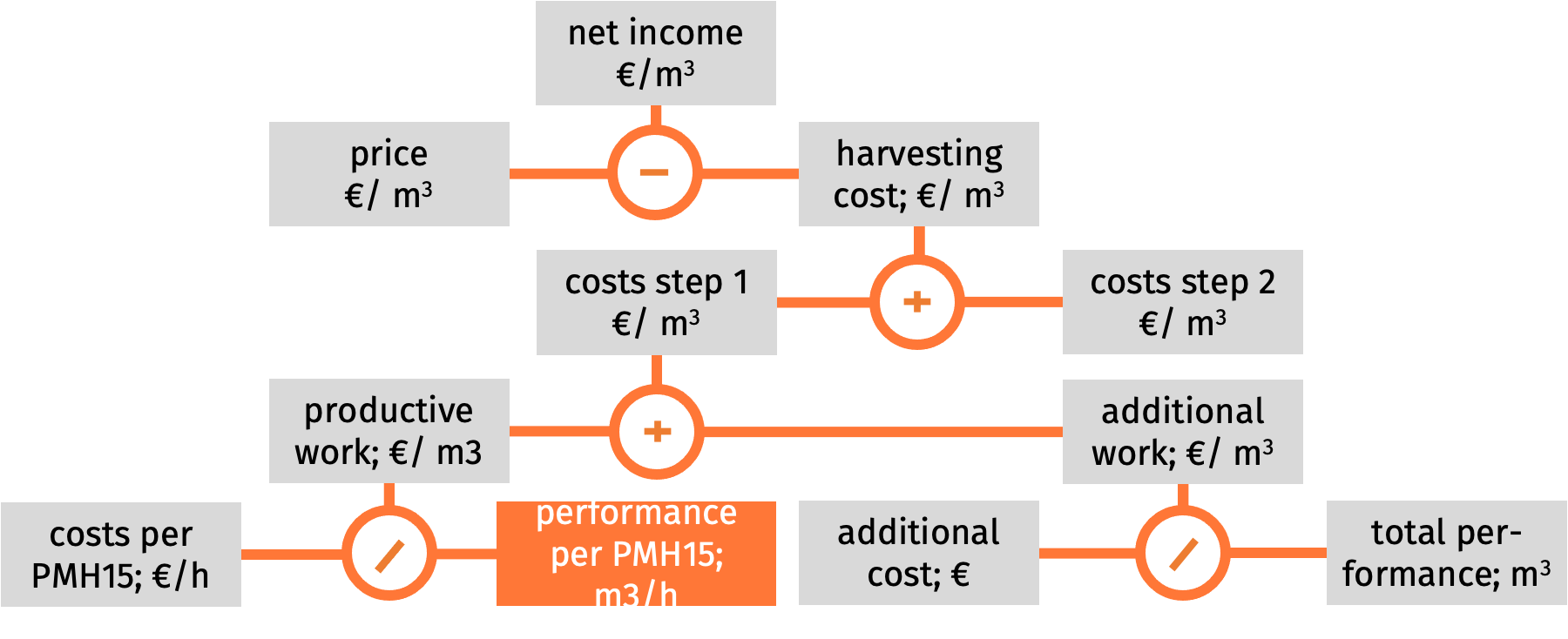
System
performance is the productivity of a working system in products per hour. In
forest harvesting, normally the products are not indicated by the trees, but by
the cubic meters (m3) that are harvested per hour.
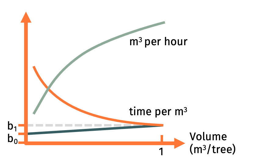
The performance
of a working system depends very much on the attributes of the working object. Besides
the tree species, the dimension of the harvested trees has a high influence to the
productivity. In scientific publications about working systems, performance is
normally represented by a typical curve (green line):
• It is low for smaller work objects
(in our case: trees)
• It increases with the work object
size according to a non-linear degressive trend.
Some graphs
also report time consumption in minutes per cubic meter (red curve). Again, we
recognize a typical curve:
• Time per cubic meter is higher for
small trees compared with big ones
• The trend is degressive.
This system
behavior is known as the principle of tree volume. The time to process a given
work object increases, but not as much as the volume of the object increases.
The problem is that we know this overall trend, but we don’t have the exact
parameters case-by-case. This makes prediction difficult and laborious.
In Technodiversity,
we suggest a simple solution: Scientific experience has shown that the time
consumption per tree depends on its volume according to a typical relationship:
• The bigger the tree, the longer the
time needed
• The data cloud can be well
represented by a linear regression
• The regression line crosses the
y-axis above the origin.
Of course,
in scientific case studies different curve types will offer a better fit, but
the linear function is fairly good, too, and gives us the chance to get an
overall estimation of the performance. This general assumption makes it
possible to forecast the system performance even with very few data points.
Provided
that we can accept the linear approximation, we can describe the relationship
between time per tree and tree size with the equation just below:
The time ti
is composed by two summands:
b0 is the fixed time
required for processing one single tree. It does not depend on the size of the
tree. It is typically the time to walk to the tree, clean the area around it
etc.
b1 is the time required for processing
a single tree. It depends on its size, so we say it is variable. b1
indicates the time consumption at one tree that has exactly the volume of 1
cubic meter. Is the tree smaller, let’s say only 0.5 m3, than the product of b1
times its volume vi is also 0.5 compared with 1 m3.
Given this
basic line, the time per m3 is
with
This curve
ti,m3 includes our two independent variables b0
and b1 with the consequence that it looks different for each
working system.
Now,
dividing 60 min/h by the time consumption ti,m3 we get the
performance in m3/h
with
and
It shows
the typical degressively increasing curve of performance (green):
• the bigger the average tree the
higher the performance per hour
• but the increment gets less and
less.
• Why do we need to complicate our
lives by tracing the process all the way back to the time consumption per tree?
• Because that way we get to the
original source of time consumption.
• We know that the relationship
between time consumption per tree and tree size can be represented by a linear
regression with two parameters b0 and b1.
Those two parameters contain all the information that we need.
• To find those parameters, very few
time measurements are enough.
• We can also modify the two
parameters of the regression formula for rough forecast purposes:
• When we see, that in our case the
preparation time b0 per tree is higher than normal (because
of thornbushes, slippery ground etc.), we can “correct” this parameter with a
best estimate.
• When we know that our operator is
quicker than an average operator, we may adapt the parameter b1
to his performance level.